Where Europe’s Banks Make Their Money

A great research article from WSJ on  how do some of the biggest banks in Europe make their money:

http://graphics.wsj.com/european-bank-earnings-2015-3q/

Where Europe’s Banks Make Their Money

A great research article from WSJ on  how do some of the biggest banks in Europe make their money:

http://graphics.wsj.com/european-bank-earnings-2015-3q/

Milton Friedman, Irving Fisher, and Greece

http://krugman.blogs.nytimes.com/2015/07/07/milton-friedman-irving-fisher-and-greece/

I continue to be amazed by how many people regard debt relief and devaluation as wild-eyed radical ideas; of course, it matters most that so many influential people in Europe share this ignorance. Anyway, for the record (and for my own future reference) I thought it would be helpful to post what Milton Friedman and Irving Fisherhad to say about the Greek disaster. OK, they weren’t writing specifically about Greece — Friedman was writing in 1950, Fisher in 1933. But their analyses ring truer than ever.

First, Friedman (why oh why isn’t there a full electronic copy of this essay online?):

Photo

Credit

That tells you everything you need to know about why “internal devaluation” has been such a costly strategy — and why the ECB’s failure to move aggressively early on to achieve and if possible surpass its 2 percent inflation target was a major contributing factor to this disaster.

Then Fisher on why austerity hasn’t even helped on the debt:

Photo

Credit

The basic story of the European periphery — not just Greece — is one of a poisonous interaction between Friedman and Fisher, which has produced incredible suffering while failing to reduce the debt/GDP ratio, which even in star pupils like Ireland and Spain is far higher than when austerity began; the only success has been in suffering long enough so that some growth has finally resumed, and they can call it vindication.

The bizarreness of the whole thing is how flaky, speculative ideas like expansionary austerity became orthodoxy, while applying the economics of Fisher and Friedman became heterodoxy bordering on Chavismo.

Liquidity preference, loanable funds, and Niall Ferguson

http://krugman.blogs.nytimes.com/2009/05/02/liquidity-preference-loanable-funds-and-niall-ferguson-wonkish/

Joe Nocera writes about Thursday’s New York Revie/PEN event on the economy, but fails to mention what I found the most depressing aspect of the whole thing: further confirmation that we’re living in aDark Age of macroeconomics, in which hard-won knowledge has simply been forgotten.

What’s the evidence? Niall Ferguson “explaining” that fiscal expansion will actually be contractionary, because it will drive up interest rates. At least that’s what I think he said; there were so many flourishes that it’s hard to tell. But in any case, this is really sad: John Hicks knew far more about this in 1937 than people who think they’re sophisticates know now.

In any case, I thought it might be useful to re-explain why our current predicament can be thought of as a global excess of desired savings — which means that fiscal deficits won’t drive up interest rates unless they also expand the economy.

Here’s what I imagine Niall Ferguson was thinking: he was thinking of the interest rate as determined by the supply and demand for savings. This is the “loanable funds” model of the interest rate, which is in every textbook, mine included. It looks like this:

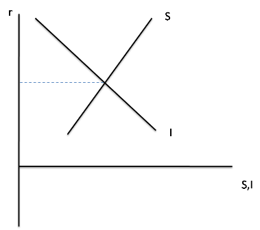
where S is savings, I investment spending, and r the interest rate.

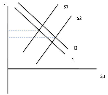
What Keynes pointed out was that this picture is incomplete if you allow for the possibility that the economy is not at full employment. Why? Because saving and investment depend on the level of GDP. Suppose GDP rises; some of this increase in income will be saved, pushing the savings schedule to the right. There may also be a rise in investment demand, but ordinarily we’d expect the savings rise to be larger, so that the interest rate falls:

So supply and demand for funds doesn’t tell you what the interest rate is — not by itself. It tells you what the interest rate would beconditional on the level of GDP; or to put it another way, it defines a relationship between the interest rate and GDP, like this:

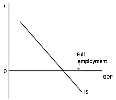
This is the IS curve, taught in Econ 101. Now, we usually explain how this curve is derived in a different way: we say that given the interest rate, you can determine investment demand, and then through the multiplier process this determines GDP. What you’re supposed to understand, however, is that the derivation I’ve just given is just a different way of arriving at the same result. It’s just different presentations of the same model.

So what determines the level of GDP, and hence also ties down the interest rate? The answer is that you need to add “liquidity preference”, the supply and demand for money. In the modern world, we often take a shortcut and just assume that the central bank adjusts the money supply so as to achieve a target interest rate, in effect choosing a point on the IS curve.

Which brings us to the current state of affairs. Right now the interest rate that the Fed can choose is essentially zero, but that’s not enough to achieve full employment. As shown above, the interest rate the Fed would like to have is negative. That’s not just what I say, by the way: the FT reports that the Fed’s own economists estimate the desired Fed funds rate at -5 percent.

What does this situation look like in terms of loanable funds? Draw the supply and demand for funds that would obtain if we were at full employment. They look like this:

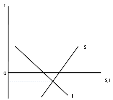
In effect, we have an incipient excess supply of savings even at a zero interest rate. And that’s our problem.

So what does government borrowing do? It gives some of those excess savings a place to go — and in the process expands overall demand, and hence GDP. It does NOT crowd out private spending, at least not until the excess supply of savings has been sopped up, which is the same thing as saying not until the economy has escaped from the liquidity trap.

Now, there are real problems with large-scale government borrowing — mainly, the effect on the government debt burden. I don’t want to minimize those problems; some countries, such as Ireland, are being forced into fiscal contraction even in the face of severe recession. But the fact remains that our current problem is, in effect, a problem of excess worldwide savings, looking for someplace to go.

IS-LMentary

taken from http://krugman.blogs.nytimes.com/2011/10/09/is-lmentary/

A number of readers, both at this blog and other places, have been asking for an explanation of what IS-LM is all about. Fair enough – this blogosphere conversation has been an exchange among insiders, and probably a bit baffling to normal human beings (which is why I have been labeling my posts “wonkish”). 

[Update: IS-LM stands for investment-savings, liquidity-money — which will make a lot of sense if you keep reading]

So, the first thing you need to know is that there are multiple correct ways of explaining IS-LM. That’s because it’s a model of several interacting markets, and you can enter from multiple directions, any one of which is a valid starting point.

My favorite of these approaches is to think of IS-LM as a way to reconcile two seemingly incompatible views about what determines interest rates. One view says that the interest rate is determined by the supply of and demand for savings – the “loanable funds” approach. The other says that the interest rate is determined by the tradeoff between bonds, which pay interest, and money, which doesn’t, but which you can use for transactions and therefore has special value due to its liquidity – the “liquidity preference” approach. (Yes, some money-like things pay interest, but normally not as much as less liquid assets.)

How can both views be true? Because we are at minimum talking about *two* variables, not one – GDP as well as the interest rate. And the adjustment of GDP is what makes both loanable funds and liquidity preference hold at the same time.

Start with the loanable funds side. Suppose that desired savings and desired investment spending are currently equal, and that something causes the interest rate to fall. Must it rise back to its original level? Not necessarily. An excess of desired investment over desired savings can lead to economic expansion, which drives up income. And since some of the rise in income will be saved – and assuming that investment demand doesn’t rise by as much – a sufficiently large rise in GDP can restore equality between desired savings and desired investment at the new interest rate.

That means that loanable funds doesn’t determine the interest rate per se; it determines a set of possible combinations of the interest rate and GDP, with lower rates corresponding to higher GDP. And that’s the IS curve.

Meanwhile, people deciding how to allocate their wealth are making tradeoffs between money and bonds. There’s a downward-sloping demand for money – the higher the interest rate, the more people will skimp on liquidity in favor of higher returns. Suppose temporarily that the Fed holds the money supply fixed; in that case the interest rate must be such as to match that demand to the quantity of money. And the Fed can move the interest rate by changing the money supply: increase the supply of money and the interest rate must fall to induce people to hold a larger quantity.

Here too, however, GDP must be taken into account: a higher level of GDP will mean more transactions, and hence higher demand for money, other things equal. So higher GDP will mean that the interest rate needed to match supply and demand for money must rise.

This means that like loanable funds, liquidity preference doesn’t determine the interest rate per se; it defines a set of possible combinations of the interest rate and GDP – the LM curve.

And that’s IS-LM:

The point where the curves cross determines both GDP and the interest rate, and at that point both loanable funds and liquidity preference are valid. 

What use is this framework? First of all, it helps you avoid fallacies like the notion that because savings must equal investment, government spending cannot lead to a rise in total spending – which right away puts us above the level of argument that famous Chicago professors somehow find convincing. And it also gets you past confusions like the notion that government deficits, by driving up interest rates, can actually cause the economy to contract.

Most spectacularly, IS-LM turns out to be very useful for thinking about extreme conditions like the present, in which private demand has fallen so far that the economy remains depressed even at a zero interest rate. In that case the picture looks like this:

Why is the LM curve flat at zero? Because if the interest rate fell below zero, people would just hold cash instead of bonds. At the margin, then, money is just being held as a store of value, and changes in the money supply have no effect. This is, of course, the liquidity trap.  

And IS-LM makes some predictions about what happens in the liquidity trap. Budget deficits shift IS to the right; in the liquidity trap that has no effect on the interest rate. Increases in the money supply do nothing at all.

That’s why in early 2009, when the WSJ, the Austrians, and the other usual suspects were screaming about soaring rates and runaway inflation, those who understood IS-LM were predicting that interest rates would stay low and that even a tripling of the monetary base would not be inflationary. 

Events since then have, as I see it, been a huge vindication for the IS-LM types – despite some headline inflation driven by commodity prices – and a huge failure for the soaring-rates-and-inflation crowd.

Yes, IS-LM simplifies things a lot, and can’t be taken as the final word. But it has done what good economic models are supposed to do: make sense of what we see, and make highly useful predictions about what would happen in unusual circumstances. Economists who understand IS-LM have done vastly better in tracking our current crisis than people who don’t.